Adaptive mutation steps#
In sequential Monte Carlo (SMC), resampling can produce many copies of the same particle. Mutation moves help these copies explore the current target distribution, but choosing how many moves to run involves a tradeoff: too few can leave the population poorly explored, while too many spend computation on moves that may add little useful exploration.
A fixed number of mutation steps may also be a poor fit throughout a run. As tempering moves from the prior towards the posterior, the target becomes more concentrated and the acceptance rate can change. This example adapts the number of attempted moves using the previous stage’s acceptance rate, aiming for a chosen number of accepted moves per particle. Lower acceptance requests more attempts at the next stage, up to a configurable limit. This provides a simple way to adjust mutation effort without choosing a separate step count for every stage. Accepted moves are only a rough guide to exploration, so the example also plots the adaptation and posterior for inspection.
adaptive_mutation_steps.py samples the same Rosenbrock likelihood
family as the basic examples, using eight dimensions by default, a normalized
uniform prior on [-5, 5]^8 and an unnormalized likelihood:
The default scale is s = rosenbrock_scale = 1. Evidence refers to this
likelihood convention; the example does not provide an analytic reference.
The likelihood reads the scale and the prior reads the bounds from
context.shared.
Setup and running#
Use Python 3.11 or later with Sequince’s plotting and HDF5 dependencies:
python -m pip install 'sequince[corner,hdf5]'
Run from the adaptive_mutation_steps directory:
python adaptive_mutation_steps.py
Edit the parameters near the top of the script to experiment. Outputs go to
outdir within this example’s directory.
Running again replaces those outputs. The example uses a seeded NumPy
generator, like the basic examples; its random stream may differ from older
versions that initialized an orng.RandomGenerator directly.
How adaptation works#
The sampler draws equal-weight particles from the prior, then repeats
adaptive tempering, systematic resampling and differential evolution mutation.
The tempering ESS target is 0.7 * n_particles; resampling runs at every
stage. Temperature adaptation and mutation-budget adaptation are separate.
Wrap the mutation step with an acceptance-based policy:
adaptive_mutation = AdaptMutationSteps(
    DifferentialEvolutionMutation(posterior),
    policy=AcceptanceRatePolicy(
        target_steps=target_steps,
        min_steps=min_steps,
        max_steps=max_steps,
    ),
    initial_steps=initial_steps,
    min_steps=min_steps,
    max_steps=max_steps,
)
target_steps=5 targets five accepted moves per particle, rather than five
attempts. Each stage executes a fixed budget, initially 5 * n_dimensions
(40 by default). After the complete block, the policy measures acceptance
a_t = n_accepted / n_attempted and selects the next budget:
Thus 50% acceptance requests ten steps next time, and 10% requests fifty.
The budget is frozen before the next mutation block starts; adaptation never
stops a block based on its own trajectory. Logs show both the completed
budget and the next decision. The final decision is unused once the sampler
reaches beta=1.
Inspect the plots and results#
The script saves:
adaptive_mutation_history.png: three panels showing executed mutation steps, observed acceptance probability, and accepted moves per particle (steps times acceptance). The dashed line marks the target of five accepted moves. Iteration numbers start at zero and match the logs. TheAdaptiveMutationPlotcallback updates this figure during the run.history.png: temperature and log evidence versus SMC iteration.corner.png: marginal and joint posterior distributions.posterior.npz: final particles, normalized weights and log evidence.result.h5: the saved SMC result, including completed mutation metrics.
Read the first two adaptation panels together: lower acceptance increases the following stage’s budget. Accepted moves need not equal the target, because acceptance changes between stages, budgets are integers and the maximum can prevent enough moves. Acceptance alone does not measure mixing or independent-sample effective sample size. Inspect the posterior and compare several seeds and particle counts before judging sampling quality.
Try lowering max_steps to see the budget saturate, or increasing
target_steps to request more mutation work. Keep
min_steps <= initial_steps <= max_steps and n_dimensions >= 2.
Retain weights when loading posterior.npz for further analysis.
Example results#
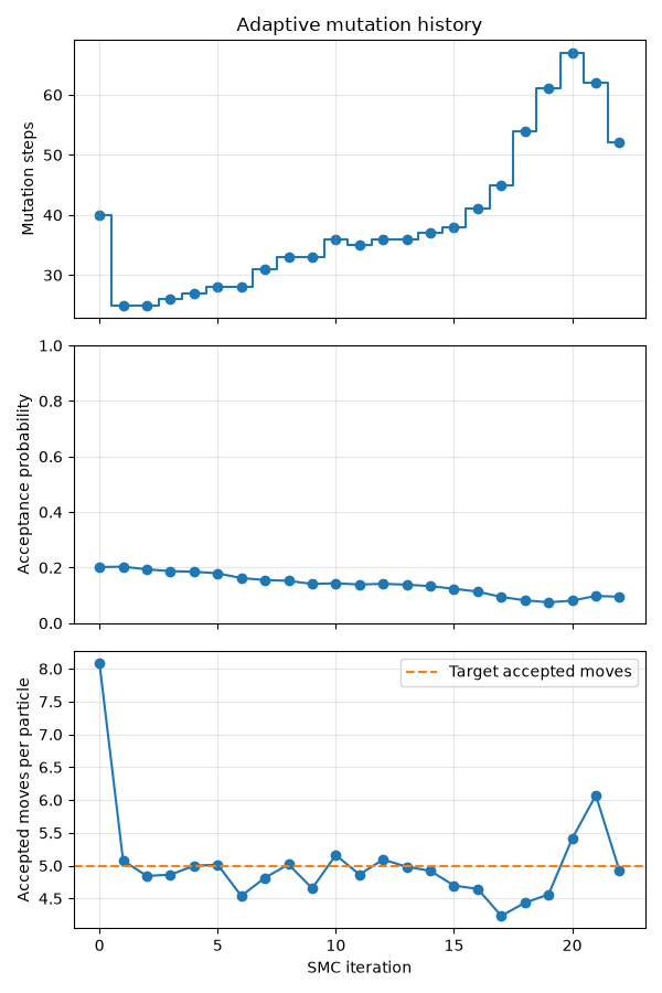
Executed mutation budgets, acceptance rates, and expected accepted moves across SMC stages.#
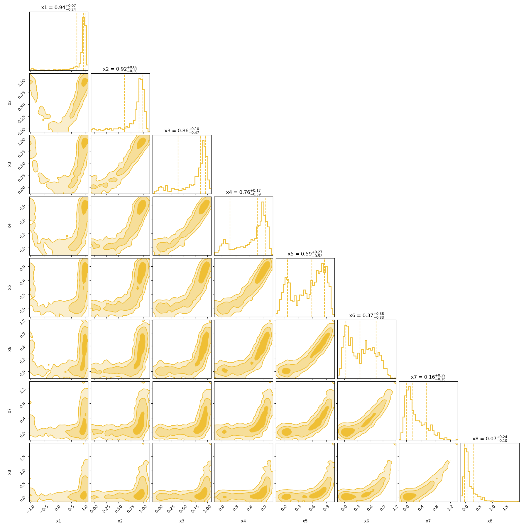
Weighted marginal and joint distributions for the eight-dimensional Rosenbrock posterior.#
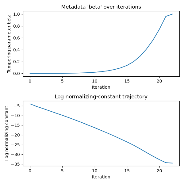
Temperature and log evidence through the adaptive mutation run.#
The full sampler setup is shown below:
  1"""Adapt mutation budgets for a Rosenbrock posterior. See README.rst."""
  2
  3from __future__ import annotations
  4
  5import logging
  6from pathlib import Path
  7
  8import matplotlib.pyplot as plt
  9import numpy as np
 10from sequince import SequentialMonteCarlo, TemperedPosterior
 11from sequince.callbacks import AdaptiveMutationPlot
 12from sequince.log import configure_logging
 13from sequince.state import ParticleState
 14from sequince.steps import (
 15    AdaptiveTemperedWeighting,
 16    AdaptMutationSteps,
 17    DifferentialEvolutionMutation,
 18    LoggingStep,
 19    StepContext,
 20    SystematicResampling,
 21)
 22from sequince.steps.mutation.adaptive.policies.acceptance import (
 23    AcceptanceRatePolicy,
 24)
 25
 26# Edit these parameters to explore the example.
 27n_particles = 1000
 28n_dimensions = 8
 29rosenbrock_scale = 1.0
 30lower_bound, upper_bound = -5.0, 5.0
 31seed = 1234
 32target_steps = 5  # Target accepted moves per particle, not attempted moves.
 33initial_steps = 5 * n_dimensions
 34min_steps, max_steps = 1, 128
 35outdir = Path("outdir")
 36
 37
 38def log_likelihood(particles: np.ndarray, context: StepContext) -> np.ndarray:
 39    """Evaluate an unnormalized Rosenbrock likelihood.
 40
 41    Parameters
 42    ----------
 43    particles : numpy.ndarray, shape (n_particles, n_dimensions)
 44        Batch of parameter vectors, with at least two dimensions.
 45    context : StepContext
 46        Runtime context containing the positive Rosenbrock scale.
 47
 48    Returns
 49    -------
 50    log_density : numpy.ndarray, shape (n_particles,)
 51        Negative Rosenbrock potential divided by the scale. Evidence uses
 52        this unnormalized likelihood convention.
 53    """
 54    scale = context.shared["rosenbrock_scale"]
 55    x = particles[..., :-1]
 56    y = particles[..., 1:]
 57    potential = np.sum(100.0 * (y - x**2.0) ** 2.0 + (1.0 - x) ** 2.0, axis=-1)
 58    return -potential / scale
 59
 60
 61def log_prior(particles: np.ndarray, context: StepContext) -> np.ndarray:
 62    """Evaluate a normalized uniform prior within the configured box.
 63
 64    Parameters
 65    ----------
 66    particles : numpy.ndarray, shape (n_particles, n_dimensions)
 67        Batch of parameter vectors.
 68    context : StepContext
 69        Runtime context whose shared mapping contains the prior bounds.
 70
 71    Returns
 72    -------
 73    log_density : numpy.ndarray, shape (n_particles,)
 74        Log prior density, with negative infinity outside the bounds.
 75    """
 76    lower = context.shared["bounds"][:, 0]
 77    upper = context.shared["bounds"][:, 1]
 78    in_bounds = np.all((particles >= lower) & (particles <= upper), axis=-1)
 79    log_volume = np.sum(np.log(upper - lower))
 80    return np.where(in_bounds, -log_volume, -np.inf)
 81
 82
 83def main() -> None:
 84    """Run adaptive SMC and save diagnostic plots, particles, and results."""
 85    logger = configure_logging(level=logging.INFO)
 86    rng = np.random.default_rng(seed)
 87    bounds = np.tile([lower_bound, upper_bound], (n_dimensions, 1))
 88    outdir.mkdir(parents=True, exist_ok=True)
 89
 90    # Define a tempered posterior with the log prior and log likelihood
 91    # functions.
 92    posterior = TemperedPosterior(
 93        log_prior=log_prior,
 94        log_likelihood=log_likelihood,
 95    )
 96
 97    # Freeze each stage's budget before mutation. Its completed acceptance
 98    # rate determines the next stage's budget, within the configured bounds.
 99    fixed_length_mutation = DifferentialEvolutionMutation(posterior)
100    adaptive_mutation = AdaptMutationSteps(
101        fixed_length_mutation,
102        policy=AcceptanceRatePolicy(
103            target_steps=target_steps,
104            min_steps=min_steps,
105            max_steps=max_steps,
106        ),
107        initial_steps=initial_steps,
108        min_steps=min_steps,
109        max_steps=max_steps,
110    )
111
112    # Define a logging function to report the current state of the SMC
113    # algorithm
114    def mutation_log_message(
115        state: ParticleState, context: StepContext
116    ) -> str:
117        """Report the completed budget and the next stage's decision."""
118        del state
119        return (
120            f"SMC iteration {context.iteration}: "
121            f"beta={context.metadata.get('beta', 0.0):.3g}, "
122            f"mutation steps={adaptive_mutation.current_n_steps}, "
123            f"next={adaptive_mutation.next_n_steps}"
124        )
125
126    # Define the SMC runner with the adaptive mutation step and logging
127    # We use the standard SMC steps: adaptive tempering, resampling, and
128    # mutation.
129    # We also add a callback to plot the adaptive mutation steps over the
130    # course of the run
131    runner = SequentialMonteCarlo(
132        steps=[
133            AdaptiveTemperedWeighting(posterior, target_ess_ratio=0.7),
134            SystematicResampling(always_resample=True),
135            adaptive_mutation,
136            LoggingStep(str_fn=mutation_log_message),
137        ],
138        callbacks=[
139            AdaptiveMutationPlot(outdir, target_steps=target_steps),
140        ],
141    )
142
143    # Define the initial state, which contains particles drawn from the prior
144    initial_particles = rng.uniform(
145        bounds[:, 0],
146        bounds[:, 1],
147        size=(n_particles, n_dimensions),
148    )
149    initial_state = ParticleState(initial_particles)
150
151    # Run the SMC algorithm with the initial state and
152    # the random number generator.
153    # We also pass in a shared context that contains the bounds and the
154    # Rosenbrock scale, which are used in the log prior and log likelihood
155    result = runner.run(
156        initial_state,
157        rng=rng,
158        shared_context={
159            "bounds": bounds,
160            "rosenbrock_scale": rosenbrock_scale,
161        },
162    )
163
164    state = result.final_state
165    logger.info("Estimated log evidence: %.4f", state.log_evidence)
166    logger.info("Posterior mean: %s", result.weighted_mean())
167    logger.info("Posterior covariance:\n%s", result.weighted_covariance())
168
169    fig = result.plot_corner(
170        parameter_labels=[f"x{i + 1}" for i in range(n_dimensions)]
171    )
172    fig.savefig(outdir / "corner.png")
173    plt.close(fig)
174
175    fig, axes = plt.subplots(2, 1, figsize=(6, 6))
176    result.plot_metadata_history("beta", ax=axes[0])
177    axes[0].set_ylabel("Tempering parameter beta")
178    result.plot_log_evidence(ax=axes[1])
179    fig.tight_layout()
180    fig.savefig(outdir / "history.png")
181    plt.close(fig)
182
183    # Keep weights with particles so subsequent analysis remains valid.
184    np.savez(
185        outdir / "posterior.npz",
186        particles=state.particles,
187        weights=state.weights,
188        log_evidence=state.log_evidence,
189    )
190    result.save_to_file(outdir / "result.h5")
191
192
193if __name__ == "__main__":
194    main()