Waste-free sequential Monte Carlo#
run_waste_free_smc.py demonstrates waste-free
sequential Monte Carlo (SMC), as described by Dau and Chopin (2022)
in Waste-free sequential Monte Carlo, alongside a
standard resample-move SMC run. Both sample a four-dimensional correlated
Gaussian likelihood with a uniform prior on [-10, 10]^4.
Run from this directory using an environment with Sequince, NumPy and Matplotlib installed:
python run_waste_free_smc.py
Wrap a mutation step to retain its full chains:
WasteFreeResampleMove(
    MetropolisHastingsMutation(posterior, GaussianRandomWalk(scale=0.7)),
    chain_length=100,
)
With N = 10,000 input particles and chain length P = 100, the waste-free
step resamples M = N / P = 100 starts, runs P - 1 = 99 transitions per
chain and retains all 100 samples, including each start and repeats after
rejection. The output has 10,000 uniformly weighted particles.
chain_length includes the start and must divide N.
For comparison, standard SMC explicitly resamples and mutates:
MultinomialResampling(always_resample=True)
MetropolisHastingsMutation(
    posterior, GaussianRandomWalk(scale=0.7), n_steps=99
)
The standard run maintains 100 particles and keeps each chain’s endpoint. Both runs use the same target, proposal, tempering ESS ratio and 100 chains with 99 transitions each per stage. This matches mutation work per stage; initial population sizes and adaptive temperature schedules differ, so stage counts and total target evaluations can differ. The script logs likelihood evaluation counts alongside posterior moments. Retained waste-free samples are correlated, and their count is not an independent-sample effective sample size. One run of each method illustrates usage, rather than establishing relative statistical efficiency.
LoggingStep reports temperature and log evidence at each stage. The
final log summary compares posterior counts, stage counts, likelihood
evaluations and evidence estimates, and quotes the retained-count ratio.
The single figure, waste_free_history.png, compares the inverse-temperature
schedules. Stage numbers match the log messages. The legend and logs quote
the final posterior counts: 100 endpoints for standard SMC and 10,000
retained samples for waste-free SMC. Both populations have uniform weights;
the larger retained count does not imply 100 times as many independent
samples.
The target has zero mean and covariance
covariance[i, j] = 0.8 ** abs(i - j). Posterior means should approach
zero and marginal variances should approach one. The evidence reference is
-4 * log(20) (approximately -11.983), neglecting the tiny Gaussian mass
outside the prior box. Both densities include their normalization constants.
Example plots#
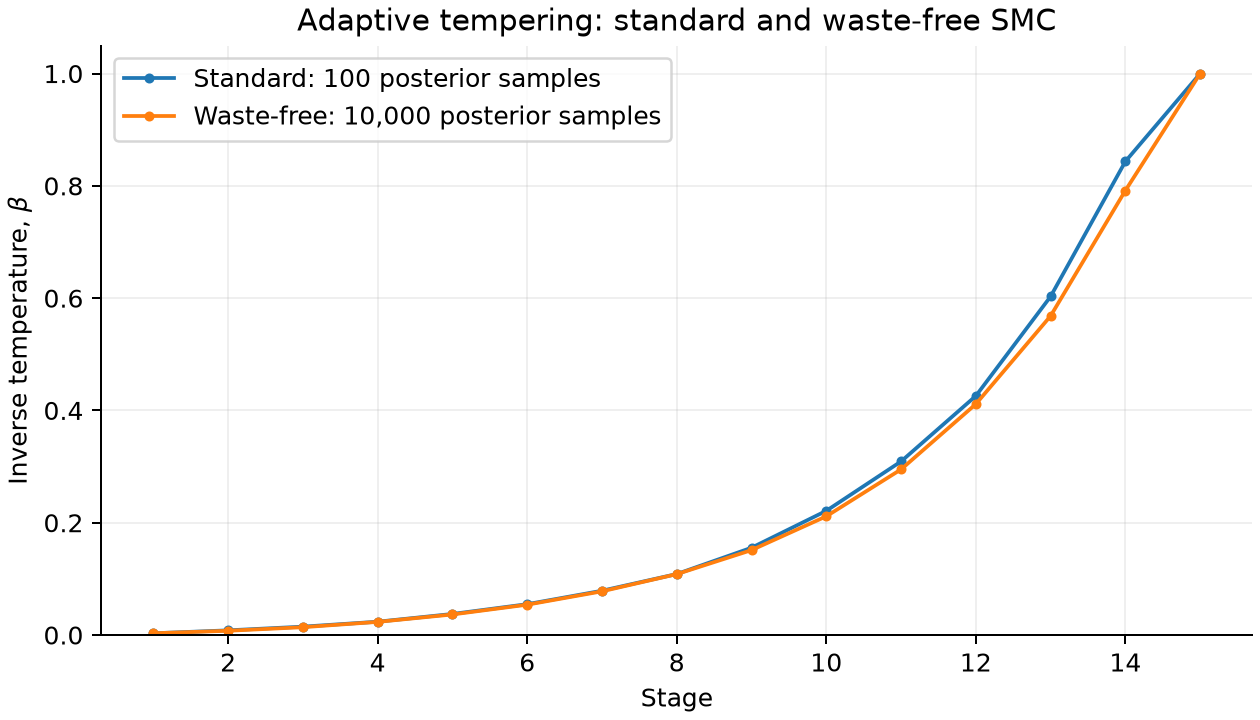
Adaptive tempering schedules for standard and waste-free SMC. Retained sample counts do not measure the number of independent samples.#
Complete script#
The target densities and complete sampler setup are shown below:
  1"""Waste-free SMC for a correlated Gaussian likelihood and uniform prior."""
  2
  3import json
  4from pathlib import Path
  5
  6import matplotlib.pyplot as plt
  7import numpy as np
  8from sequince import ParticleState, SequentialMonteCarlo, TemperedPosterior
  9from sequince.log import configure_logging
 10from sequince.steps import (
 11    AdaptiveTemperedWeighting,
 12    LoggingStep,
 13    MultinomialResampling,
 14    StepContext,
 15    WasteFreeResampleMove,
 16)
 17from sequince.steps.mutation import (
 18    GaussianRandomWalk,
 19    MetropolisHastingsMutation,
 20)
 21
 22dims = 4
 23bounds = (-10.0, 10.0)
 24correlation = 0.8
 25n_chains = 100
 26chain_length = 100  # Includes the resampled starting state.
 27seed = 123
 28documentation_output: Path | None = None
 29
 30
 31def log_likelihood(particles: np.ndarray, context: StepContext) -> np.ndarray:
 32    """Return normalized zero-mean Gaussian log densities."""
 33    whitened = np.linalg.solve(context.shared["cholesky"], particles.T)
 34    return context.shared["log_norm"] - 0.5 * np.sum(whitened**2, axis=0)
 35
 36
 37def log_prior(particles: np.ndarray, context: StepContext) -> np.ndarray:
 38    """Return normalized uniform log densities inside the prior box."""
 39    lower, upper = context.shared["bounds"]
 40    inside = np.all((particles >= lower) & (particles <= upper), axis=1)
 41    return np.where(
 42        inside, -particles.shape[1] * np.log(upper - lower), -np.inf
 43    )
 44
 45
 46def main() -> None:
 47    logger = configure_logging()
 48    indices = np.arange(dims)
 49    covariance = correlation ** np.abs(indices[:, None] - indices[None, :])
 50    cholesky = np.linalg.cholesky(covariance)
 51    log_norm = (
 52        -0.5 * dims * np.log(2 * np.pi) - np.log(np.diag(cholesky)).sum()
 53    )
 54    posterior = TemperedPosterior(log_prior, log_likelihood)
 55    # Truncation at +/-10 has negligible effect on the evidence reference.
 56    reference_log_evidence = -dims * np.log(bounds[1] - bounds[0])
 57    logger.info("Reference log evidence: %.4f", reference_log_evidence)
 58    fig, ax = plt.subplots(figsize=(7, 4), layout="constrained")
 59    comparison_rows: list[str] = []
 60    posterior_counts: dict[str, int] = {}
 61
 62    summaries: dict[str, dict] = {}
 63
 64    for name in ("Standard", "Waste-free"):
 65        mutation = MetropolisHastingsMutation(
 66            posterior,
 67            GaussianRandomWalk(scale=0.7),
 68            n_steps=chain_length - 1,
 69        )
 70        if name == "Waste-free":
 71            n_particles = n_chains * chain_length
 72            moves = [
 73                WasteFreeResampleMove(mutation, chain_length=chain_length)
 74            ]
 75        else:
 76            n_particles = n_chains
 77            moves = [MultinomialResampling(always_resample=True), mutation]
 78
 79        logger.info("%s SMC: %d particles", name, n_particles)
 80        rng = np.random.default_rng(seed)
 81        initial = ParticleState(rng.uniform(*bounds, size=(n_particles, dims)))
 82        smc = SequentialMonteCarlo(
 83            steps=[
 84                AdaptiveTemperedWeighting(posterior, target_ess_ratio=0.85),
 85                *moves,
 86                LoggingStep(
 87                    str_fn=lambda state, context: (
 88                        f"Stage {context.t + 1}: "
 89                        f"beta={float(context.metadata['beta']):.4f}, "
 90                        f"log evidence={float(state.log_evidence):.4f}"
 91                    )
 92                ),
 93            ]
 94        )
 95        results = smc.run(
 96            initial,
 97            rng=rng,
 98            shared_context={
 99                "bounds": bounds,
100                "cholesky": cholesky,
101                "log_norm": log_norm,
102            },
103        )
104        particles = results.final_state.particles
105        logger.info(
106            "%s posterior means (reference: zero): %s",
107            name,
108            particles.mean(axis=0),
109        )
110        logger.info(
111            "%s posterior variances (reference: one): %s",
112            name,
113            particles.var(axis=0),
114        )
115        if documentation_output is not None:
116            summaries[name] = {
117                "log_evidence": float(results.final_state.log_evidence),
118                "weighted_mean": results.weighted_mean().tolist(),
119                "weighted_population_covariance": results.weighted_covariance().tolist(),
120                "n_particles": len(particles),
121                "likelihood_evaluations": int(
122                    results.context.evaluation_counts.log_likelihood_evaluations
123                ),
124            }
125        posterior_counts[name] = len(particles)
126        comparison_rows.append(
127            f"{name:<12} {len(particles):>10,d} {len(results.outputs):>8d} "
128            f"{results.context.evaluation_counts.log_likelihood_evaluations:>16,d} "
129            f"{float(results.final_state.log_evidence):>12.4f}"
130        )
131        stages = np.arange(1, len(results.outputs) + 1)
132        ax.plot(
133            stages,
134            results.metadata_history("beta"),
135            marker=".",
136            label=f"{name}: {len(particles):,} posterior samples",
137        )
138
139    logger.info(
140        "Final comparison:\n%-12s %10s %8s %16s %12s\n%s",
141        "Method",
142        "Samples",
143        "Stages",
144        "Likelihood evals",
145        "Log evidence",
146        "\n".join(comparison_rows),
147    )
148    logger.info(
149        "Waste-free retains %.0f times as many posterior samples; "
150        "these samples are correlated, including repeats after rejection.",
151        posterior_counts["Waste-free"] / posterior_counts["Standard"],
152    )
153
154    ax.set(
155        title="Adaptive tempering: standard and waste-free SMC",
156        xlabel="Stage",
157        ylabel=r"Inverse temperature, $\beta$",
158        ylim=(0, 1.05),
159    )
160    ax.spines[["top", "right"]].set_visible(False)
161    ax.grid(alpha=0.2)
162    ax.legend()
163    output_directory = documentation_output or Path(".")
164    fig.savefig(output_directory / "waste_free_history.png", dpi=180)
165    if documentation_output is not None:
166        (documentation_output / "summary.json").write_text(
167            json.dumps(summaries, allow_nan=False) + "\n"
168        )
169    plt.close(fig)
170    logger.info("Saved waste_free_history.png")
171
172
173if __name__ == "__main__":
174    main()