Gaussian posterior#

These examples walk through Bayesian inference with Sequince’s standard Sequential Monte Carlo (SMC) sampler. Start with gaussian.py to learn the workflow, then run rosenbrock.py to explore a curved posterior and customize mutation and resampling. Each script contains its own prior, likelihood, and sampler setup. Edit the parameters near the top of the script to experiment.

Setup and running#

Use Python 3.11 or later and install Sequince with the optional plotting and HDF5 dependencies:

python -m pip install 'sequince[corner,hdf5]'

For installation options, including using a development checkout, see “Getting started” in the main Sequince documentation.

Run the script from this directory:

python gaussian.py

The script writes to outdir/gaussian within this directory. Running a script again replaces its previous outputs.

1. Define the target distribution#

Sequince needs functions that evaluate the log prior and log likelihood. Both receive a batch of particles with shape (n_particles, n_dimensions) and a StepContext, and return one value per particle, with shape (n_particles,). Sequince passes the context when evaluating the target. Use context.shared to read static model parameters supplied to smc.run through shared_context. For example, both scripts define the prior as:

def log_prior(particles, context):
    lower_bound = context.shared["lower_bound"]
    upper_bound = context.shared["upper_bound"]
    inside = np.all(
        (particles >= lower_bound) & (particles <= upper_bound), axis=-1
    )
    log_density = -particles.shape[1] * np.log(upper_bound - lower_bound)
    return np.where(inside, log_density, -np.inf)

The Gaussian likelihood reads mean and sigma from the same shared mapping; the Rosenbrock likelihood reads its coefficients a and b. This makes the target functions independent of module-level model settings.

For a parameter vector \(\boldsymbol{\theta}\) with \(d\) dimensions, the examples use independent uniform priors between -5 and 5:

\[\begin{split}\log p(\boldsymbol{\theta}) = \begin{cases} -d \log 10, & \boldsymbol{\theta} \in [-5, 5]^d, \\ -\infty, & \text{otherwise}. \end{cases}\end{split}\]

Including the prior normalization is necessary for a correct evidence estimate.

In gaussian.py, the likelihood is a standard multivariate Gaussian, including its normalization constant (the defaults are mean=0 and sigma=1). The resulting posterior is a standard Gaussian restricted to the prior box. Its mean is zero, and its covariance is very close to the identity for these wide bounds. The script also computes the analytic evidence, including the Gaussian probability mass inside the box.

2. Initialize particles from the prior#

Create a seeded NumPy generator, draw particles from the prior, and put them in a ParticleState:

rng = np.random.default_rng(seed)
initial_state = ParticleState(
    particles=rng.uniform(
        lower_bound, upper_bound, size=(n_particles, n_dimensions)
    ),
)

When log_weights is omitted, ParticleState supplies equal normalized weights, each with log weight \(\log w_i = -\log N\), where \(N\) is the number of particles (n_particles). This is appropriate here because the particles are drawn from the prior, the initial target distribution. There is no need to set the weights explicitly. Supply log_weights when constructing a state that already has nonuniform importance weights.

Keep using the same generator for the sampler. Changing the initialization to a different distribution requires accounting for that proposal; see the main API reference for make_standard_bayesian_smc and its log_proposal option.

3. Configure the sampler#

Use the prebuilt helper to assemble the standard Bayesian SMC workflow:

smc, posterior, metadata = make_standard_bayesian_smc(
    log_prior=log_prior,
    log_likelihood=log_likelihood,
    target_ess_ratio=0.8,
    mutation="minipcn",
    mutation_n_steps=16,
)

The sampler moves through tempered distributions

\[\pi_\beta(\boldsymbol{\theta}) \propto p(\boldsymbol{\theta})\,L(\boldsymbol{\theta})^\beta, \qquad 0 \leq \beta \leq 1,\]

where \(p\) is the prior and \(L\) is the likelihood. It starts at the prior with \(\beta=0\) and finishes at the posterior with \(\beta=1\). Adaptive tempering chooses increments using an effective sample size (ESS) criterion. Resampling concentrates particles in regions of higher weight, and mutation moves help the population explore each intermediate distribution.

The helper returns the SMC runner, a tempered posterior object, and initial metadata. These scripts use the runner and metadata directly; the posterior object is also available for further sampling with draw_additional_samples. See “Configuring the runner” in the main User guide and the helper’s API reference for resampling thresholds, mutation choices, and other options.

4. Run SMC#

Pass the initial population, generator, and helper metadata to the runner:

result = smc.run(
    initial_state,
    rng=rng,
    shared_context={
        "lower_bound": lower_bound,
        "upper_bound": upper_bound,
        "mean": mean,
        "sigma": sigma,
    },
    metadata=metadata,
)

The runner makes shared_context available as context.shared in both target functions. The Gaussian example supplies the bounds, mean, and standard deviation shown above; the Rosenbrock example supplies bounds and its two coefficients. Treat this mapping as read-only during the run.

The helper’s metadata is available as context.metadata and carries evolving information such as the tempering parameter \(\beta\) (context.metadata["beta"]). Sequince’s tempered posterior applies \(\beta\) to the likelihood; the likelihood functions return their ordinary log likelihood, without applying \(\beta\) themselves. context.t identifies the current SMC iteration. The configured sampler stops when it reaches the posterior. Logging shows progress and the running evidence estimate.

See “Meta data & shared context” in the main Getting started guide and “Working with particle state” in the User guide for these interfaces.

5. Inspect and save the result#

result.final_state contains the final particles, their weights, and the log evidence estimate. result.weighted_mean() and result.weighted_covariance() compute posterior summaries using those weights. For the Gaussian, compare the summaries and evidence with the known values. Monte Carlo estimates fluctuate; agreement improves with adequate particles and mixing, rather than being exact for a single run.

Each script saves:

corner.png: marginal and joint posterior plots.
history.png: the tempering parameter and log evidence over iterations.
posterior.npz: particles, normalized weights, and the log evidence estimate.
result.h5: the SMC result saved using result.save_to_file.

The arrays can be loaded with numpy.load. Retain the weights when analyzing the particles. See the main API reference for SMCResult for posterior sample extraction, diagnostics, plotting, and result persistence.

Gaussian results#

Download script.

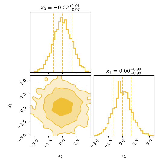
Weighted marginal and joint posterior distributions for the Gaussian target.#

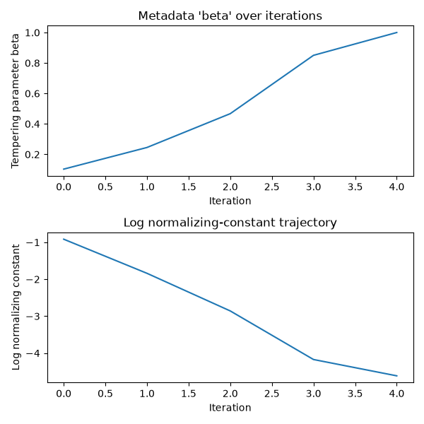
Adaptive temperature and accumulated log evidence at each SMC stage.#

Run provenance.

"""Sample a Gaussian posterior using Sequince. See README.rst."""

import logging
from math import erf, sqrt
from pathlib import Path

import matplotlib.pyplot as plt
import numpy as np
from sequince import ParticleState, make_standard_bayesian_smc
from sequince.log import configure_logging
from sequince.steps import StepContext

# Edit these parameters to explore the example.
n_dimensions = 2
n_particles = 2000
lower_bound, upper_bound = -5.0, 5.0
mean, sigma = 0.0, 1.0
seed = 42
outdir = Path("outdir/gaussian")


def log_prior(particles: np.ndarray, context: StepContext) -> np.ndarray:
    """Evaluate a normalized uniform prior within the bounds.

    Parameters
    ----------
    particles : numpy.ndarray, shape (n_particles, n_dimensions)
        Batch of parameter vectors.
    context : StepContext
        Runtime context whose shared mapping contains the model parameters.

    Returns
    -------
    log_density : numpy.ndarray, shape (n_particles,)
        Log prior density, with negative infinity outside the bounds.
    """
    lower_bound = context.shared["lower_bound"]
    upper_bound = context.shared["upper_bound"]
    inside = np.all(
        (particles >= lower_bound) & (particles <= upper_bound), axis=-1
    )
    log_density = -particles.shape[1] * np.log(upper_bound - lower_bound)
    return np.where(inside, log_density, -np.inf)


def log_likelihood(particles: np.ndarray, context: StepContext) -> np.ndarray:
    """Evaluate a normalized Gaussian likelihood.

    Parameters
    ----------
    particles : numpy.ndarray, shape (n_particles, n_dimensions)
        Batch of parameter vectors.
    context : StepContext
        Runtime context whose shared mapping contains the model parameters.

    Returns
    -------
    log_density : numpy.ndarray, shape (n_particles,)
        Gaussian log density for each particle.
    """
    mean = context.shared["mean"]
    sigma = context.shared["sigma"]
    return -0.5 * np.sum(((particles - mean) / sigma) ** 2, axis=-1) - (
        0.5 * particles.shape[1] * np.log(2.0 * np.pi * sigma**2)
    )


def main() -> None:
    """Sample the posterior and save particles, plots, and the SMC result."""
    configure_logging(level=logging.INFO)
    rng = np.random.default_rng(seed)
    outdir.mkdir(parents=True, exist_ok=True)

    # ParticleState supplies equal weights, appropriate for prior draws.
    initial_state = ParticleState(
        particles=rng.uniform(
            lower_bound, upper_bound, size=(n_particles, n_dimensions)
        ),
    )

    # The helper combines adaptive tempering, resampling, and mutation moves.
    smc, posterior, metadata = make_standard_bayesian_smc(
        log_prior=log_prior,
        log_likelihood=log_likelihood,
        target_ess_ratio=0.8,
        mutation="minipcn",
        mutation_n_steps=16,
    )
    result = smc.run(
        initial_state,
        rng=rng,
        shared_context={
            "lower_bound": lower_bound,
            "upper_bound": upper_bound,
            "mean": mean,
            "sigma": sigma,
        },
        metadata=metadata,
    )

    state = result.final_state
    print(f"Estimated log evidence: {state.log_evidence:.4f}")
    # Include the Gaussian mass within the finite prior bounds.
    prior_mass = 0.5 * (
        erf((upper_bound - mean) / (sigma * sqrt(2.0)))
        - erf((lower_bound - mean) / (sigma * sqrt(2.0)))
    )
    log_evidence = n_dimensions * (
        np.log(prior_mass) - np.log(upper_bound - lower_bound)
    )
    print(f"Analytic log evidence:  {log_evidence:.4f}")
    print(f"Untruncated Gaussian mean: {mean}; variance: {sigma**2}.")
    print(f"Posterior mean: {result.weighted_mean()}")
    print(f"Posterior covariance:\n{result.weighted_covariance()}")

    fig = result.plot_corner()
    fig.savefig(outdir / "corner.png")
    plt.close(fig)

    fig, axes = plt.subplots(2, 1, figsize=(6, 6))
    result.plot_metadata_history("beta", ax=axes[0])
    axes[0].set_ylabel("Tempering parameter beta")
    result.plot_log_evidence(ax=axes[1])
    fig.tight_layout()
    fig.savefig(outdir / "history.png")
    plt.close(fig)

    # Keep weights with the particles so subsequent analysis remains valid.
    np.savez(
        outdir / "posterior.npz",
        particles=state.particles,
        weights=state.weights,
        log_evidence=state.log_evidence,
    )
    result.save_to_file(outdir / "result.h5")


if __name__ == "__main__":
    main()

Continue with Rosenbrock posterior to explore a curved posterior and conditional resampling.

Gaussian posterior

Contents