Flow preconditioning

sequince supports preconditioning for mutation steps, as described by Karamanis et al. (2022). A normalizing flow can learn a transformation from the current particle population to a simpler latent space, where the mutation kernel can explore more efficiently.

sequince.transforms.FlowTransform adapts a normalizing flow for use as a particle transform. The flow must implement the sequince.flows.NormalizingFlow protocol:

Construct the transform by passing it a compatible flow and, optionally, the keyword arguments used to fit that flow:

from sequince.transforms import FlowTransform

flow = ...
preconditioning_transform = FlowTransform(
    flow=flow,
    fit_kwargs={...},
)

The resulting object can be used anywhere a particle transform is accepted by sequince.

Fitting the flow

The fitting of the transform is handled by the mutation step. The frequency of fitting can be controlled by the transform_refit argument. Current options are:

• "always": fit the flow every time the mutation step is called (default)

• "once": fit the first time the mutation step is called, then reuse

• "per-context": fit once per unique context, then reuse for that context

When using the prebuilt samplers, the transform_refit argument should be passed in the mutation_kwargs dictionary.

Prebuilt flows

sequince-density provides various normalizing flows that can be used for preconditioning via the zuko and flowjax packages. See the sequince_density.flows.zuko and sequince_density.flows.flowjax modules for more information.

Continue with Persistent sampling to combine this approach with persistent sampling.

Example

The following example uses a Zuko masked autoregressive flow to precondition a four-dimensional Rosenbrock target. It requires sequince-density with its Zuko backend and PyTorch support.

Example plots

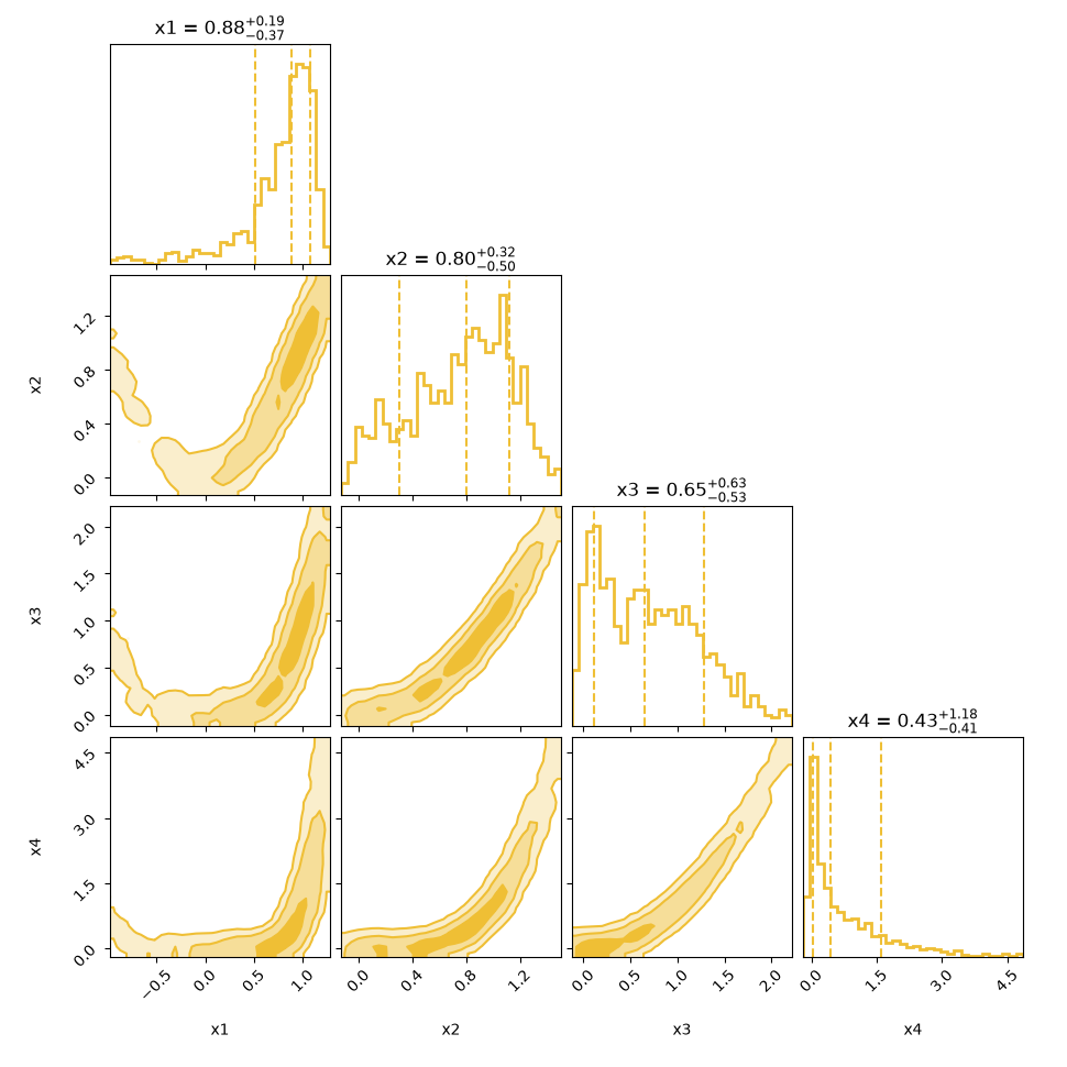
Posterior marginals and joint distributions for the four-dimensional Rosenbrock target sampled with flow preconditioning.

Run provenance.

Download the script.

"""Example of using a normalizing flow for preconditioning in sequince.

Running this example requires the sequince-density package to be installed with
the zuko backend.
"""

from __future__ import annotations

import json
import logging
from pathlib import Path

import numpy as np
import torch
from orng import RandomGenerator
from sequince.array_api import to_numpy
from sequince.callbacks import IntermediateParticlesPlot, ParticleTransformPlot
from sequince.log import configure_logging
from sequince.plot import plot_corner
from sequince.prebuilt_samplers import make_standard_bayesian_smc
from sequince.result import SMCResult
from sequince.state import ParticleState
from sequince.transforms import AffineTransform, FlowTransform
from sequince_density.flows.zuko import ZukoFlow

seed = 1234
n_particles = 1000
dims = 4
rosenbrock_scale = 1.0
outdir = Path("./")
documentation_output: Path | None = None


def rosenbrock(x: torch.Tensor) -> torch.Tensor:
    return torch.sum(
        100.0 * (x[..., 1:] - x[..., :-1] ** 2.0) ** 2.0
        + (1.0 - x[..., :-1]) ** 2.0,
        dim=-1,
    )


def log_prior(particles: torch.Tensor, context) -> torch.Tensor | float:
    lower = context.shared["bounds"][:, 0]
    upper = context.shared["bounds"][:, 1]
    in_bounds = torch.all((particles >= lower) & (particles <= upper), dim=-1)
    log_volume = torch.sum(torch.log(upper - lower))
    values = torch.where(in_bounds, -log_volume, -torch.inf)
    return values


def log_likelihood(particles: torch.Tensor, context) -> torch.Tensor | float:
    potential = rosenbrock(particles)
    values = -potential / context.shared["rosenbrock_scale"]
    return values


def _documentation_summary(result: SMCResult) -> dict[str, object]:
    """Summarize the weighted empirical measure on the host for JSON output."""
    state = result.final_state
    particles = to_numpy(state.particles)
    weights = to_numpy(state.weights)
    mean = np.sum(particles * weights[:, None], axis=0) / weights.sum()
    centered = particles - mean
    # The pinned Sequince revision uses a NumPy-only transpose signature in
    # weighted_covariance. Host arrays keep this documentation step portable.
    covariance = (centered * weights[:, None]).T @ centered / weights.sum()
    return {
        "log_evidence": float(state.log_evidence),
        "weighted_mean": mean.tolist(),
        "weighted_population_covariance": covariance.tolist(),
        "n_particles": len(particles),
    }


def main() -> None:
    logger = configure_logging(level=logging.INFO)

    rng = RandomGenerator(backend="torch", seed=seed)

    bounds = torch.tensor([[-5.0, 5.0]]).repeat(dims, 1)
    labels = [f"x{i + 1}" for i in range(dims)]

    # Define the normalizing flow to use for preconditioning.
    # We use a Masked Autoregressive Flow (MAF) with 2 transforms and 2 hidden
    # layers of 16 units each.
    flow = ZukoFlow(
        dims=bounds.shape[0],
        flow_class="MAF",
        transforms=2,
        hidden_features=[16, 16],
        particle_transform=AffineTransform(),
        seed=seed,
    )

    # We then construct a preconditioning transform that uses the flow to
    # transform the particles. This transform will be applied to the particles
    # before the mutation step in the SMC algorithm.
    # We also specify some fitting parameters for the flow.
    transform = FlowTransform(
        flow=flow, fit_kwargs={"n_epochs": 75, "lr": 5e-3, "batch_size": 128}
    )

    # Construct the SMC sampler with the preconditioning transform.  We use the
    # default settings for the SMC sampler, except that we specify the
    # particle transform.
    # We also add two callbacks to plot the particles and transformed particles
    # at each iteration.
    runner, posterior, metadata = make_standard_bayesian_smc(
        log_prior=log_prior,
        log_likelihood=log_likelihood,
        particle_transform=transform,
        callbacks=[
            IntermediateParticlesPlot(
                outdir=outdir / "particles",
                base_filename="particles",
            ),
            ParticleTransformPlot(
                outdir=outdir / "particles",
                base_filename="transformed_particles",
            ),
        ],
    )

    # Draw initial particles from a uniform distribution over the bounds.
    initial_particles = rng.uniform(
        bounds[:, 0], bounds[:, 1], size=(n_particles, bounds.shape[0])
    )
    initial_state = ParticleState(initial_particles)

    # Define shared context to pass to the log_prior and log_likelihood
    # functions.
    shared_context = {
        "bounds": bounds,
        "rosenbrock_scale": rosenbrock_scale,
    }

    # Run the SMC sampler
    result = runner.run(
        initial_state,
        rng=rng,
        metadata=metadata,
        shared_context=shared_context,
    )

    if documentation_output is not None:
        summary = _documentation_summary(result)
        (documentation_output / "summary.json").write_text(
            json.dumps(summary, allow_nan=False) + "\n"
        )

    # Compute the log evidence and its standard deviation from the SMC result.
    log_evidence = result.log_evidence()
    log_evidence_std = result.log_evidence_error()
    logger.info(f"Log evidence: {log_evidence:.4f} ± {log_evidence_std:.4f}")

    # Get posterior samples and weights for plotting
    # When using rejection sampling, the weights will be uniform for accepted
    # samples.
    posterior_samples, weights = result.posterior_samples(method="rejection")

    # Plot the posterior samples
    plot_corner(
        posterior_samples,
        weights=weights,
        parameter_labels=labels,
        filename=outdir / "rosenbrock_corner.png",
    )


if __name__ == "__main__":
    main()