Rosenbrock posterior

Start with Gaussian posterior for the prior, particle initialization, and standard SMC workflow. This example keeps the same uniform prior and uses a curved likelihood with differential-evolution mutation and conditional resampling.

Run from this directory with the same dependencies as the Gaussian example:

python rosenbrock.py

Outputs are written to outdir/rosenbrock.

Define the likelihood

rosenbrock.py follows the same workflow with a Rosenbrock log likelihood:

\[\log L(\boldsymbol{\theta}) = -\sum_{j=1}^{d-1} \left[b\left(\theta_{j+1} - \theta_j^2\right)^2 + \left(a - \theta_j\right)^2\right].\]

The likelihood reads \(a\) and \(b\) from context.shared. With the default \(a=1\) and \(b=100\), the two-dimensional likelihood concentrates around a narrow curved valley near \(\theta_2 = \theta_1^2\), with a maximum at \((\theta_1, \theta_2) = (1, 1)\). Inspect the corner plot for this shape and the history plot for how tempering progresses. This likelihood is unnormalized: the reported evidence uses exactly the convention above, and the script provides no analytic reference value.

Configure mutation and resampling

The Rosenbrock example also demonstrates more options in the prebuilt helper:

smc, posterior, metadata = make_standard_bayesian_smc(
    log_prior=log_prior,
    log_likelihood=log_likelihood,
    weighting_criterion="cess",
    target_ess_ratio=0.8,
    resampling="stratified",
    always_resample=False,
    resampling_ess_threshold=0.5,
    mutation="differential-evolution",
    mutation_n_steps=32,
    mutation_kwargs={"gamma_one_probability": 0.1},
)

mutation="differential-evolution" proposes moves using scaled differences between other particles in the ensemble. mutation_kwargs passes options to the mutation implementation: here gamma_one_probability=0.1 gives each proposal a 10% chance of using a unit scale instead of the usual dimension-dependent scale. Each mutation stage takes 32 steps.

resampling="stratified" changes the resampling scheme from the Gaussian example’s default systematic scheme. With always_resample=False, resampling occurs when the population ESS falls below \(0.5N\). By default, resample_at_end=True also resamples at the final posterior, even if that threshold has not been crossed. When omitted, always_mutate follows the resolved always_resample value, so mutation runs only on iterations that resample here. Set always_mutate=True to run mutation every iteration.

Use weighting_criterion="cess" with conditional resampling. Conditional ESS (CESS) measures the effect of a proposed temperature increment given the current weighted population; target_ess_ratio=0.8 controls that increment. The separate resampling_ess_threshold=0.5 controls when to resample using the population ESS. Sequince’s ordinary "ess" tempering criterion requires resampling every iteration, so simply setting always_resample=False with that criterion is invalid.

See the main API reference for make_standard_bayesian_smc and DifferentialEvolutionMutation for the available options.

Try changing n_particles, mutation_n_steps, and the seed to assess the stability of the posterior summaries. Increasing target_ess_ratio usually produces smaller tempering increments and more iterations. Increasing particle count or mutation steps increases computational cost. Compare several runs before judging whether a setting explores the posterior adequately.

Rosenbrock results

Download script.

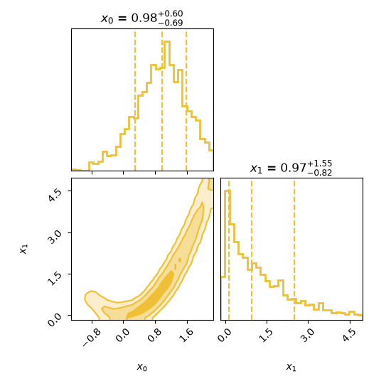
Weighted posterior samples along the curved Rosenbrock valley.

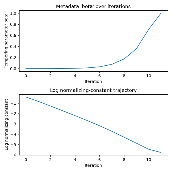
Temperature and log evidence for the unnormalized Rosenbrock likelihood.

Run provenance.

"""Sample a Rosenbrock posterior using Sequince. See README.rst."""

import logging
from pathlib import Path

import matplotlib.pyplot as plt
import numpy as np
from sequince import ParticleState, make_standard_bayesian_smc
from sequince.log import configure_logging
from sequince.steps import StepContext

# Edit these parameters to explore the example.
n_dimensions = 2
n_particles = 2000
lower_bound, upper_bound = -5.0, 5.0
a, b = 1.0, 100.0
seed = 42
outdir = Path("outdir/rosenbrock")


def log_prior(particles: np.ndarray, context: StepContext) -> np.ndarray:
    """Evaluate a normalized uniform prior within the bounds.

    Parameters
    ----------
    particles : numpy.ndarray, shape (n_particles, n_dimensions)
        Batch of parameter vectors.
    context : StepContext
        Runtime context whose shared mapping contains the model parameters.

    Returns
    -------
    log_density : numpy.ndarray, shape (n_particles,)
        Log prior density, with negative infinity outside the bounds.
    """
    lower_bound = context.shared["lower_bound"]
    upper_bound = context.shared["upper_bound"]
    inside = np.all(
        (particles >= lower_bound) & (particles <= upper_bound), axis=-1
    )
    log_density = -particles.shape[1] * np.log(upper_bound - lower_bound)
    return np.where(inside, log_density, -np.inf)


def log_likelihood(particles: np.ndarray, context: StepContext) -> np.ndarray:
    """Evaluate an unnormalized Rosenbrock likelihood.

    Parameters
    ----------
    particles : numpy.ndarray, shape (n_particles, n_dimensions)
        Batch of parameter vectors, with at least two dimensions.
    context : StepContext
        Runtime context containing Rosenbrock coefficients ``a`` and ``b``.

    Returns
    -------
    log_density : numpy.ndarray, shape (n_particles,)
        Negative Rosenbrock function values. No likelihood normalization
        constant is included, so evidence refers to this convention.
    """
    a = context.shared["a"]
    b = context.shared["b"]
    return -np.sum(
        b * (particles[:, 1:] - particles[:, :-1] ** 2) ** 2
        + (a - particles[:, :-1]) ** 2,
        axis=-1,
    )


def main() -> None:
    """Sample the posterior and save particles, plots, and the SMC result."""
    configure_logging(level=logging.INFO)
    rng = np.random.default_rng(seed)
    outdir.mkdir(parents=True, exist_ok=True)

    # ParticleState supplies equal weights, appropriate for prior draws.
    initial_state = ParticleState(
        particles=rng.uniform(
            lower_bound, upper_bound, size=(n_particles, n_dimensions)
        ),
    )

    # CESS-based tempering allows weights to accumulate between resampling.
    smc, posterior, metadata = make_standard_bayesian_smc(
        log_prior=log_prior,
        log_likelihood=log_likelihood,
        weighting_criterion="cess",
        target_ess_ratio=0.8,
        resampling="stratified",
        always_resample=False,
        resampling_ess_threshold=0.5,
        mutation="differential-evolution",
        mutation_n_steps=32,
        mutation_kwargs={"gamma_one_probability": 0.1},
    )
    result = smc.run(
        initial_state,
        rng=rng,
        shared_context={
            "lower_bound": lower_bound,
            "upper_bound": upper_bound,
            "a": a,
            "b": b,
        },
        metadata=metadata,
    )

    state = result.final_state
    print(f"Estimated log evidence: {state.log_evidence:.4f}")

    print(f"Posterior mean: {result.weighted_mean()}")
    print(f"Posterior covariance:\n{result.weighted_covariance()}")

    fig = result.plot_corner()
    fig.savefig(outdir / "corner.png")
    plt.close(fig)

    fig, axes = plt.subplots(2, 1, figsize=(6, 6))
    result.plot_metadata_history("beta", ax=axes[0])
    axes[0].set_ylabel("Tempering parameter beta")
    result.plot_log_evidence(ax=axes[1])
    fig.tight_layout()
    fig.savefig(outdir / "history.png")
    plt.close(fig)

    # Keep weights with the particles so subsequent analysis remains valid.
    np.savez(
        outdir / "posterior.npz",
        particles=state.particles,
        weights=state.weights,
        log_evidence=state.log_evidence,
    )
    result.save_to_file(outdir / "result.h5")


if __name__ == "__main__":
    main()